There is nothing from my first stats course that I remember more clearly than Prof. Asgharian repeating “I have seen what I should have seen” to describe the idea behind maximum likelihood theory. Given a family of models, maximum likelihood estimation consists of finding which values of the parameters maximize the probability of observing the dataset we have observed. This idea, popularized in part by Sir Ronald A. Fisher, profoundly changed the field of statistics at a time when access to data wasn’t at all like today. In their book Computer Age Statistical Inference: Algorithms, Evidence, and Data Science (Chapter 7), Bradley Efron and Trevor Hastie write:

If Fisher had lived in the era of “apps,” maximum likelihood estimation might have made him a billionaire.

What makes the maximum likelihood estimator (MLE) so useful is that it is consistent (converges in probability to the value it estimates) and efficient (no other estimator has lower asymptotic mean squared error). But watch out, these are statements about the MLE’s asymptotic ($n \to \infty$) behaviour when the dimension is held fixed. The story is quite different in the finite-sample situation and this is what Stein’s paradox reminds us of: in some circumstances, the MLE is bound to be (potentially grossly) sub-optimal. Hence Hastie’s and Efron’s claim: “maximum likelihood estimation has shown itself to be an inadequate and dangerous tool in many twenty-first-century applications. […] unbiasedness can be an unaffordable luxury when there are hundreds or thousands of parameters to estimate at the same time.” So who is Stein and what is Stein’s paradox? Read on.

Stein’s paradox is attributed to Charles Stein (1920-2016), an American mathematical statistician who spent most of his career at Stanford University. Stein is remembered by his colleagues not only for his exceptional work, but also for his strong belief in basic human rights and passionate social activism. In an interview by Y.K. Leong, the very first question touched his statistical work (verifying weather broadcasts for understanding how weather might affect wartime activities) for the Air Force during World War II; Stein’s first words are unequivocal:

First I should say that I am strongly opposed to war and to military work. Our participation in World War II was necessary in the fight against fascism and, in a way, I am ashamed that I was never close to combat. However, I have opposed all wars by the United States since then and cannot imagine any circumstances that would justify war by the United States at the present time, other than very limited defensive actions.

According to Stanford News, the man who was called the “Einstein of the Statistics Department”, was also the first Stanford professor arrested for protesting apartheid and was often involved in anti-war protests.

On the math-stat side, Stein is the author of a very influential/controversial paper entitled Inadmissibility of the Usual Estimator for the Mean of a Multivariate Normal Distribution (1956). To understand what it is about, we need to understand what it means for an estimator to be admissible, which is a statement about its performance. For the purpose, let us use Stein’s setup where $X = (X_1,X_2,X_3)$ is such that each component $X_i$ is independent and normally distributed, that is $X_i \sim N(\theta_i,1)$. Assessing the performance of an estimator $\hat\theta(X) = \hat\theta = (\hat\theta_1,\hat\theta_2,\hat\theta_3)$ usually involves a loss function $ L(\hat\theta, \theta) $, whose purpose is to quantify how much $\hat\theta$ differs from the true value $\theta$ it estimates. The loss function that interested Stein was the (very popular) squared Euclidean distance `$$ L(\hat\theta(X), \theta) = ||\hat\theta - \theta ||^2 = \sum_i (\hat\theta_i - \theta_i)^2.

$$ Assessing the performance of$\hat\theta$directly with$L$has the disadvantage of depending on the observed data$X$. We overcome such limitation by taking the expectation of$L(\hat\theta(X),\theta)$over$X$, that is we consider $$

R(\hat\theta, \theta) = \mathbb{E}_X\ L(\hat\theta(X), \theta).

$$ This latter is called the mean squared error, and this is what we try to minimize. An estimator$\hat\theta$is deemed inadmissible when there exists at least one estimator$\hat\vartheta$for which$R(\hat\theta, \theta) \geq R(\hat\vartheta, \theta)$for all$\theta$, with the equality being strict for at least one value of$\theta$`. In other words, an estimator is inadmissible if and only if there exists another estimator that dominates it.

Stein showed that, for the normal model, the “usual estimator”, which is the MLE, not only isn’t always the best (in terms of mean squared error), but never is the best! In their 1977 paper Stein’s Paradox in Statistics (where the term “Stein’s paradox” seems to have appeared for the first time), Bradley Efron and Carl Morris loosely described it as follows:

The best guess about the future is usually obtained by computing the average of past events. Stein’s paradox defines circumstances in which there are estimators better than the arithmetic average.

In the normal model discussed, the MLE is the arithmetic average: for iid observations $Z_1,Z_2,Z_3 \sim N(\vartheta,1)$, the MLE of $\vartheta$ is $\sum_i Z_i/3$. Stein’s setup is a little different in that each variable $X_i$ has its own location parameter $\theta_i$, and so the MLE of $(\theta_1,\theta_2,\theta_3)$ simply is $(X_1,X_2,X_3)$. Now, since the variables are independent, it seems natural to think that this is the best estimator we can find. After all, the groups are totally unrelated. Well well, nope. As long as we consider three different location parameters $\theta_i$ or more, we can do better! Or, to put it differently, the MLE is optimal only when we consider one or two unique location parameters.

In 1961, a few years after the publication of Inadmissibility, Stein and his graduate student, Willard James, strengthened the argument in Estimation with quadratic loss. They provided an explicit estimator out-performing the MLE. Hastie and Efron highlight this as an important moment in the history of statistics: “It begins the story of shrinkage estimation, in which deliberate biases are introduced to improve overall performance, at a possible danger to individual estimates.”

For the rest of the post, I focus on a concrete application of Stein’s theory. In that department, there’s nothing like the famous baseball example of Efron and Morris, which first appeared in their 1975 paper Data Analysis Using Stein’s Estimator and its Generalizations. The example involves the batting averages (number of hits/number of times at bat) of 18 major-league baseball players. During the 1970 season, when top batter Roberto Clemente had appeared 45 times at bat, seventeen other players had $n=45$ times at bat. The first column (Hits/AB) of the following table provides the batting averages for the eighteen players in question (reproduced with Professor Efron’s permission, whom we would like to thank):

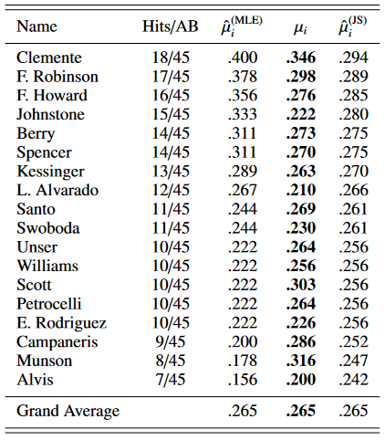
Let us go back in time and suppose we are at this exact date in 1970. To predict the batting averages of each player for the remainder of the season, it seems natural (with no other information) to use their current batting averages. Again, this coincides with the MLE under the normal model, and this is why the column labeled $\hat\mu_i^{(\mathrm{MLE})}$ simply shows the same ratios, this time in decimal form.

To get a glimpse of why the MLE is sub-optimal, define a class of estimators parametrized by $c$ as follows: let $\hat\mu^{(c)} = (\hat\mu_{1}^{(c)}, \dots, \hat\mu_{18}^{(c)})$ where ` $$

\hat\mu_{i}^{(c)} = \bar{\mu} + c(\hat\mu_i^{(\mathrm{MLE})} - \bar{\mu}),

$$ and$\bar{\mu}$is the average of all means, *i.e.* the grand mean. In our case, $$

\bar{\mu} = \frac{1}{18} \sum_{i=1}^{18} \hat\mu_i^{(\mathrm{MLE})}

$$ is the overall batting average of the$d=18$players. Note that$\hat\mu^{(MLE)} = \hat\mu^{(1)}$, and so the MLE is indeed part of the class of estimators we consider. Now, define the James-Stein estimator as the one minimizing the mean squared error, that is$\hat\mui^{(JS)} = \hat\mu{i}^{(c^*)}$for $$

c^* := {\rm argmin}_{c \in [0,1]}\ R(\hat\mu^{©}, \mu),

$$ where$\mu = (\mu1, \dots, \mu{18})$represents the *true/ideal* batting averages of the players (may they exist) that we are trying to estimate. As the definition of$\hat\mu^{©}$` suggests, Stein’s method consists of shrinking the individual batting average of each player towards their grand average: in Efron’s and Morris’ words,

if a player’s hitting record is better than the grand average, then it must be reduced; if he is not hitting as well as the grand average, then his hitting record must be increased.

If the MLE $\hat\mu_i^{(\mathrm{MLE})}$ were to minimize the mean squared error $R(\hat\mu^{(c)}, \mu)$, it would mean $c^* = 1$. This is where Stein’s result comes into play: it states that if $c^*$ minimizes the mean squared error, then it must be the case that $c^*<1$ and so $\hat\mu^{(\mathrm{JS})} \neq \hat\mu^{(\mathrm{MLE})}$.

The method proposed by James and Stein (1961) to estmimate $c^*$ leads to the value $c^*=.212$, and since in our example the grand average is $\bar\mu = .265$, we get ` $$

\hat\mu_i^{(\mathrm{JS})} = .265 + (.212)(\hat\mu_i^{(\mathrm{MLE})} - .265)

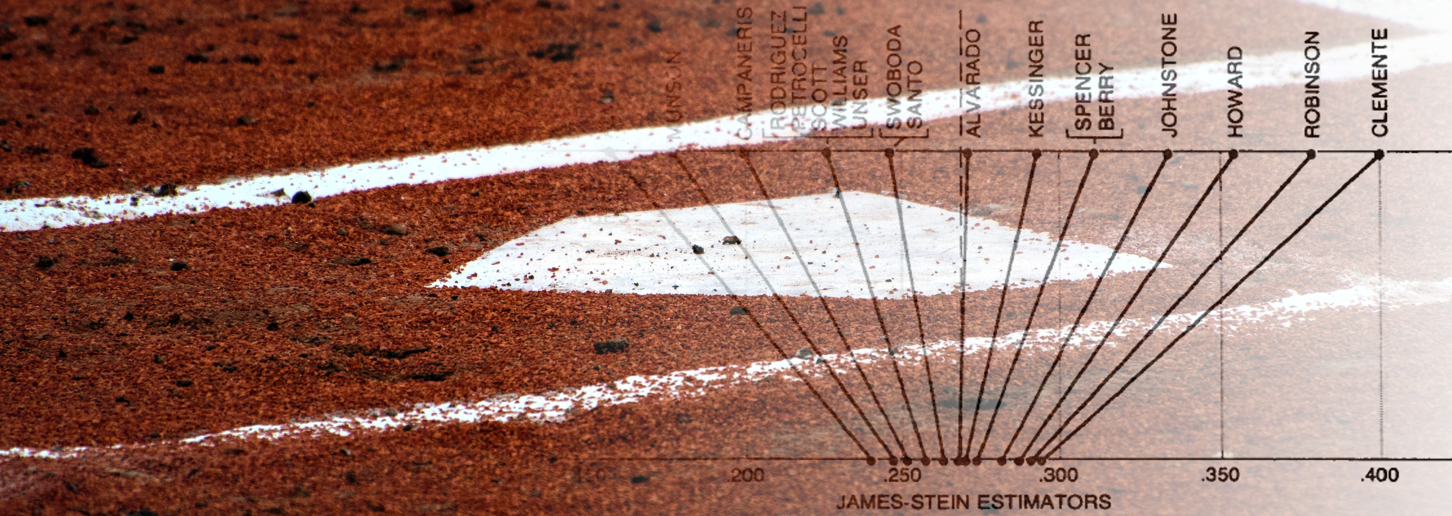
$$ ` Efron and Morris provide a very intuitive illustration of the effect of shrinkage in this particular example.

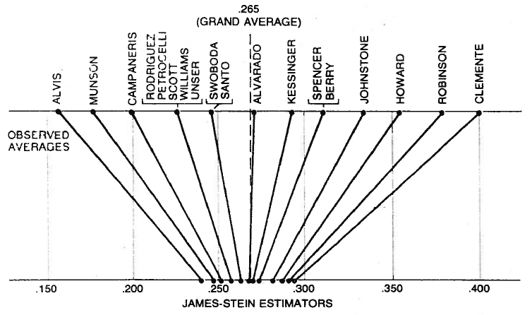
As we can see, everyone is pulled by the grand average of batting averages. Coming back to 2018, let us look at what actually happened during the remainder of the 1970 season. The table’s bold column provides the batting averages computed for the rest of the season. Let us say that those, which were often computed on more than 200 (new) times at bat, are good approximations of the true/ideal batting averages. It turns out that, for 16 of the 18 players, $\hat\mu_i^{(\mathrm{JS})}$ actually does a better job than $\hat\mu_i^{(\mathrm{MLE})}$ at predicting $\mu_i$. It does a better job in terms of total squared error as well.

It can seem puzzling that, to estimate Clemente’s batting average (the highest), using Alvis’ batting average (the lowest) should help. According to our formulas, if Alvis’ batting average $\hat\mu_{\mathrm{Alvis}}^{(\mathrm{MLE})}$ was different, then our guess $\hat\mu_{\mathrm{Clemente}}^{(\mathrm{JS})}$ for Clemente would be different as well (because $\bar\mu$ would be different).

It becomes more intuitive when you realize that the value of $c^*$ actually depends on $n$, the number of observations available to us (times at bat in our example). As $n$ increases, the optimal value $c^*$ gets closer to $1$, and so less shrinkage is applied. Stein’s Theorem states that $c^*<1$ no matter what; yet, it might be very close to one, and so $\hat\mu_{i}^{(\mathrm{MLE})}$ and $\hat\mu_{i}^{(\mathrm{JS})}$ might be extremely similar.

This last property of the James-Stein estimator is similar to that of bayesian estimators, which relies more and more on the data (and less on the prior distribution) as the number of observations increases. Indeed, Efron and Morris identified Stein’s method, designed under a strictly frequentist regime, as an empirical Bayes rule (inference procedures where the prior is estimated from the data as well, instead of being set by the user). For more details on Stein’s Paradox and its relation to empirical Bayes methods, I recommend the book Computer Age Statistical Inference: Algorithms, Evidence, and Data Science by Efron and Hastie, which provides, among many otherthings, a nice historical perspective of modern methods used by statisticians and a gentle introduction to the connections and disagreements relating and opposing the two main statistical theories: frequentism and bayesianism.

I have to give some credit to Laurent Caron, Stéphane Caron and Simon Youde for their useful comments on preliminary versions of the post.

$$